
Results
|
|
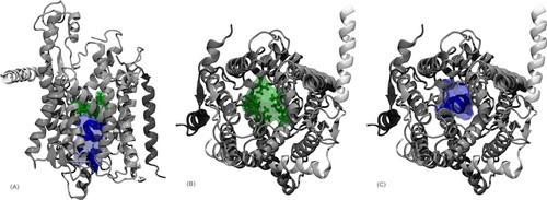
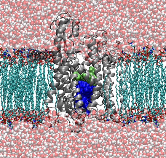
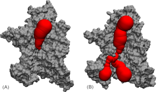
An example for such a natural membrane channel is the protein-conducting channel SecYEβ. Here, proteins are both translocated across and inserted into the membrane. Two of the main structural features of this protein channel are a pore region, consisting of a ring of six hydrophobic residues located in the center of the channel, as well as a "plug" consisting of a short α-helix located just below the pore region (Fig. 1).
For protein translocation, the plug has to be removed from the pore region and the pore has to be dilated. Both features guarantee the correct functionality, meaning specific transport of polypeptides through the channel area while blocking the channel in the closed state. Due to the available atomic crystal structure of the SecYEβ complex from Methanococcus jannashii, which was resolved in 2004 [1], it became possible to perform all-atom MD-simulations on this protein conducting channel.
From analysis of EM data of a protein conducting channel complex from a different species (Sec61) alone and bound to a ribosome it is speculated that association of a ribosome leads to conformational rearrangements of the protein conducting channel that in turn loosen the binding of the plug and facilitate the opening of Sec61 toward the membrane [2-4].Using newer EM data in combination with the available crystal structure it was possible to propose a model structure of a Sec61 complex bound to a ribosome in both an inactive (2AKI) and an active (2AKH) form [5].
In this work, all-atom molecular dynamics simulations are performed on both the inactive and active conformation of the protein conducting channel SecYEβ to understand the overall mechanism of protein transport across the membrane and to address questions concerning translocation, sealing of the channel and relaxation. Differences between the inactive and the active form are of particular interest in this context.
|
|
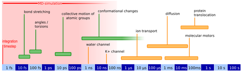
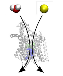
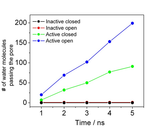
The above mentioned processes like the opening mechanism, translocation of polypeptides and other molecular components all take place on timescales which are not yet readily available to standard molecular dynamics simulations (Figure 2).
It is therefore necessary to accelerate these events during the simulation using efficient sampling schemes like SMD (Steered Molecular Dynamics) [6]. From the resulting nonequilibrium data the important equilibrium values like for example the change in free energy can then be extracted using fluctuation theorems.
|
|
In 1997, Jarzynski formulated an integral version of the fluctuation theorem, connecting the free energy difference to an exponential average of the external work [7], where W is the external work along a trajectory and angle, brackets denote the ensemble average over N trajectories. For infinite sampling of work values, the free energy estimate is exact, for finite sampling it allows an estimate of this value. This is highly dependent on how good the distribution of work values can be described.
Figure 3A shows work profiles from multiple trajectories where the system is not in equilibrium. The average work is shown in light gray and is larger than the
|
|
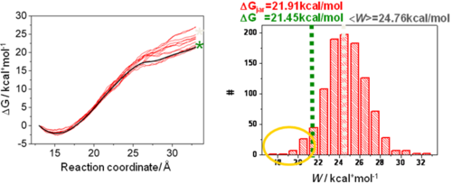
The exponential average of the work in the Jarzynski equation is mainly determined by trajectories with small work values (yellow circle in Figure 3B). These trajectories are rare events, which makes the exponential average very difficult to estimate accurately from a small number of trajectories and for systems driven far out of equilibrium due to insufficient sampling and leads to an overestimation of the free energy change.
|
|
In MD-simulations of larger biomolecules, where in general only a small number of trajectories is affordable, direct application of the Jarzynski equation is practical only for a narrow work distribution, with a width σW ≈ kBT) [8]. An approximation can be found by expanding the right side of equation (1) into a series of cumulants Cn(z) entwickelt.
The cumulants Cn(z) in equation (2) describe the shape of the work distribution, e.g. C1=〈w〉 is the mean work, C2=〈w2〉-〈w〉2 the variance of the distribution. For the special case of a Gaussian shaped work distribution, third and higher order cumulants are identically zero. In this case, only the mean and the variance of the work distribution must be estimated which can be done even for a smaller number of trajectories with acceptable statistical errors.
Additional Pictures
|
|
|
|
|
|
|
|
References
[1] van den Berg, B., et al., X-ray structure of a protein-conducting channel. Nature, 2004. 427 (6969): p. 36-44.
[2] Beckmann, R., et al., Alignment of conduits for the nascent polypeptide chain in the Ribosome-Sec61 complex. Science, 1997. 278 (5346): p. 2123-2126.
[3] Breyton, C., et al., Three-dimensional structure of the bacterial protein-translocation complex SecYEG. Nature, 2002. 418 (6898): p. 662-665.
[4] Menetret, J.F., et al., The structure of ribosome-channel complexes engaged in protein translocation. Molecular Cell, 2000. 6 (5): p. 1219-1232.
[5] Mitra, K., et al., Structure of the E-coli protein-conducting channel bound to a translating ribosome. Nature, 2005. 438 (7066): p. 318-324.
[6] Isralewitz, B., M. Gao, and K. Schulten. 2001. Steered Molecular Dynamics and Mechanical Functions of Proteins. Curr. Opin. Struc. Biol. 11: 224-230.
[7] Jarzynski, C. 1997. Nonequilibrium Equality for Free Energy Differences. Phys. Rev. Lett. 78: 2690-2693.
[8] Park, S. and K. Schulten, Calculating potentials of mean force from steered molecular dynamics simulations. Journal of Chemical Physics, 2004. 120 (13): p. 5946-5961.